Constant Acceleration Motion

Section 2.7 Constant Acceleration Motion

The one-dimensional constant acceleration motion has many applications in practice. For instance, almost all problems of freely falling bodies near Earth is first done by assuming a constant acceleration. As we have done in this chapter, we will remain with one-dimensional situations, e.g., motion along a Cartesian axis, say the \(x\) axis.

🔗

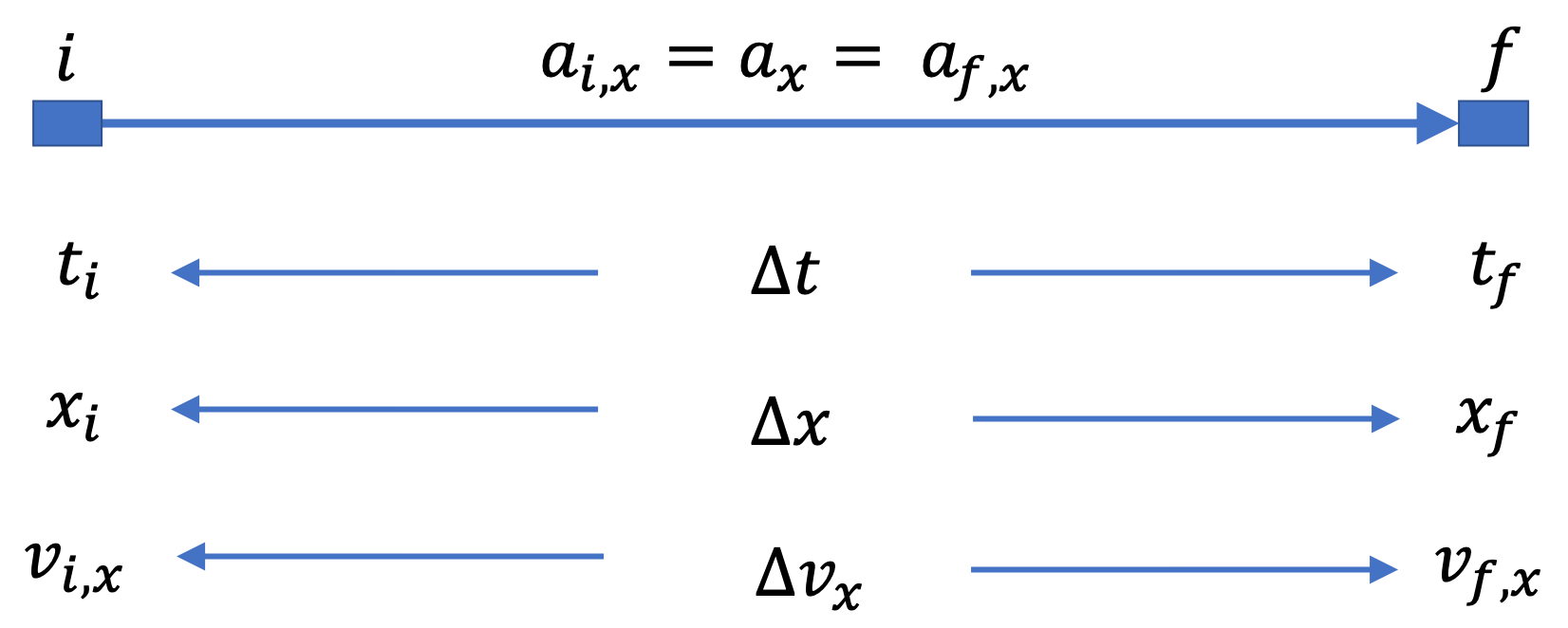
Figure 2.57 illustrates a common setup for a constant-acceleration prblems. We denote the interval by \(\Delta t = t_f - t_i \text{,}\) the change in position by \(\Delta x = x_f-x_i \text{,}\) and change in velocity by \(\Delta v_x = v_{f,x} - v_{i,x} \text{.}\) In these problems, we are typically interested in change in position and velocity over some interval of time. We do not care about what happens AT OTHER INSTANTS as long as acceleration is same at all those instants.

🔗

Figure 2.57. Set up for constant acceleration motion along the \(x \) axis with unchanging \(a_x \) throughout the interval, i.e., constant acceleration along \(x\) axis. Here, subscript \(i\) refers to initial instant and \(f\) to the final instant.
🔗

🔗

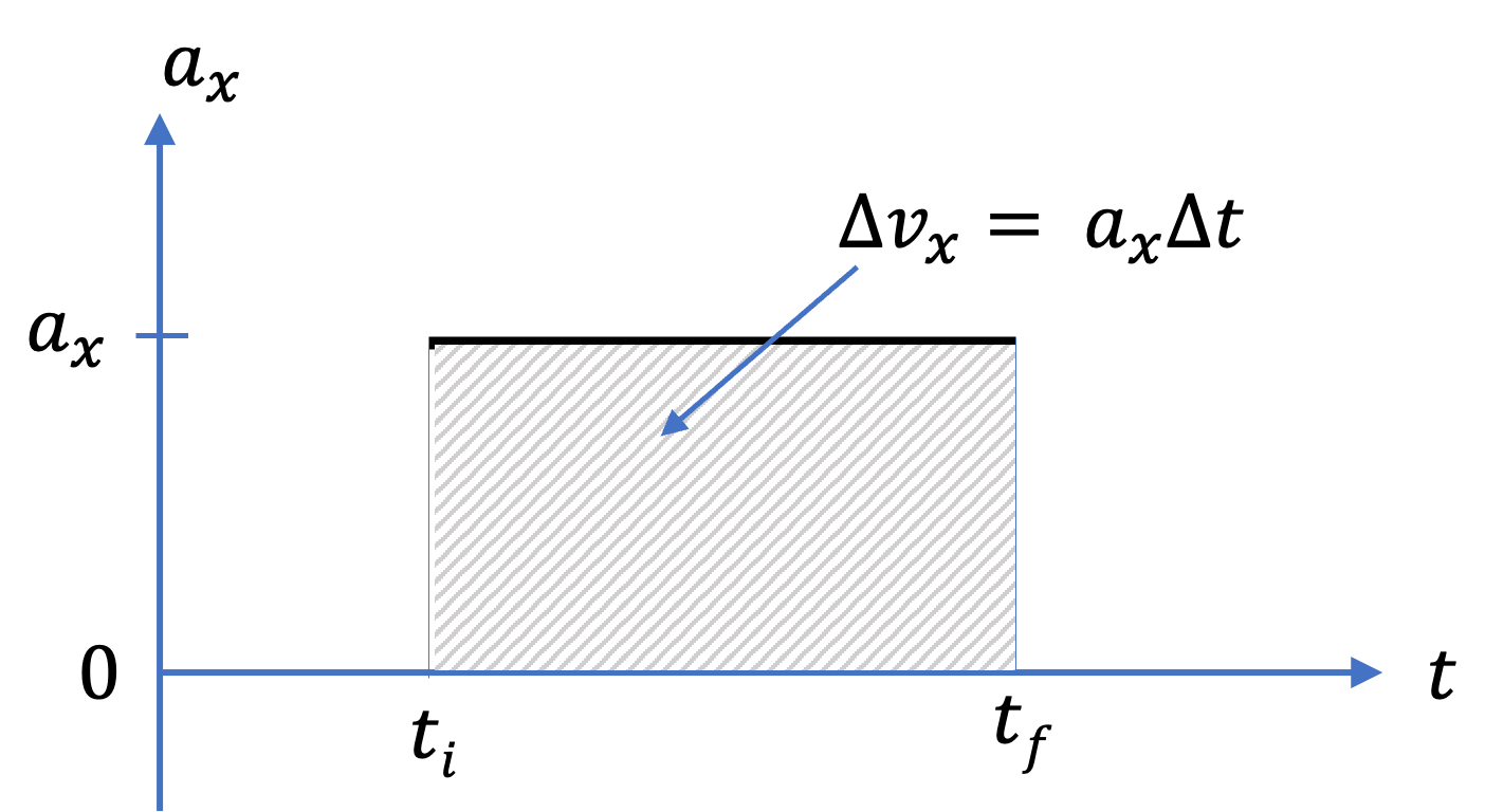
Since acceleration is constant during the interval, the change in velocity will simply be the product of acceleration and the duration.

\begin{equation} \Delta v_x = a_x \Delta t.\tag{2.14} \end{equation}

🔗

You can easily see from either thinking in terms of average acceleration or in terms of area-under-the-curve of \(a_x\) versus \(t\) as shown in Figure 2.58 or integral of a constant \(a_x\text{.}\) You can also write Eq. (2.14) more explicitly to get the following equation.

\begin{equation} v_{f,x} = v_{i,x} + a_x \left( t_f - t_i \right).\tag{2.15} \end{equation}

This formula for \(v_{f,x}\) will be same for any arbitrary instant \(t\) as the final instant. Let us denote by \(t\) the time at any arbitrary instant and \(v_x\) velocity at this arbitrary instant. Then.

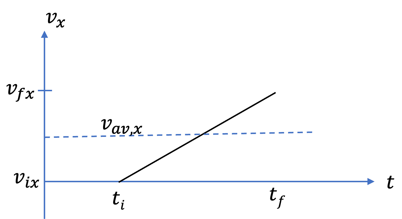
\begin{equation} v_{x} = v_{i,x} + a_x \left( t - t_i \right).\tag{2.16} \end{equation}

This says that velocity changes linearly with time, i.e., \(v_x(t)\) is a linear polynomial of \(t\text{,}\) i.e., a plot of \(v_x\) against time \(t\) will be a straight line.

\begin{equation*} v_x(t) = A + B t, \end{equation*}

with

\begin{equation*} A = v_{i,x} - a_x t_i,\ \ \ B = a_x. \end{equation*}

🔗

Therefore, average velocity will simply be the average of initial and final velocities. This is correct only in the case of constant acceleration.

\begin{equation} v_{\text{av},x} = \dfrac{v_{i,x} + v_{f,x}}{2}. \tag{2.17} \end{equation}

🔗

Now, displacement can be given just by the product of average velocity and duration. Therefore,

\begin{equation} \Delta x = v_{\text{av},x} \, \Delta t. \tag{2.18} \end{equation}

🔗

It is possible to eliminate \(\Delta t \) from these equations to obtain

\begin{equation} v_{f,x}^2 = v_{i,x}^2 + 2 a_x \left( \Delta x \right)^2,\tag{2.19} \end{equation}

which we will refer to as the “no-\(t\)-equation”. It is also possible to eliminate \(v_{f,x} \) to obtain another useful equation:

\begin{equation} \Delta x = v_{i,x} \Delta t + \dfrac{1}{2}a_x\left(\Delta t \right)^2,\tag{2.20} \end{equation}

which we will refer to as the “no-\(v_f\)-equation”.

🔗

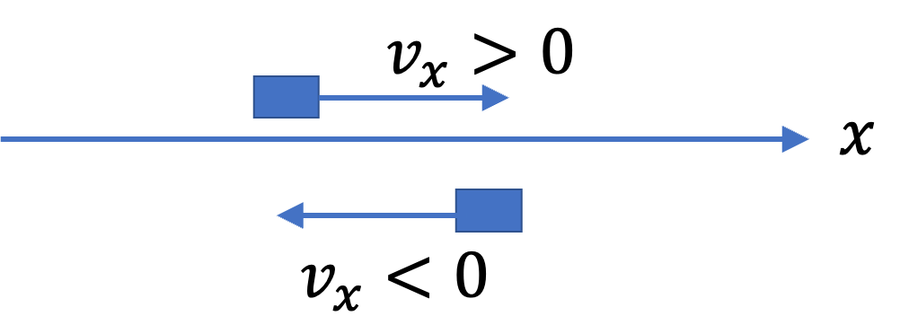
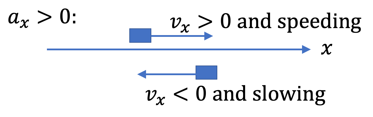
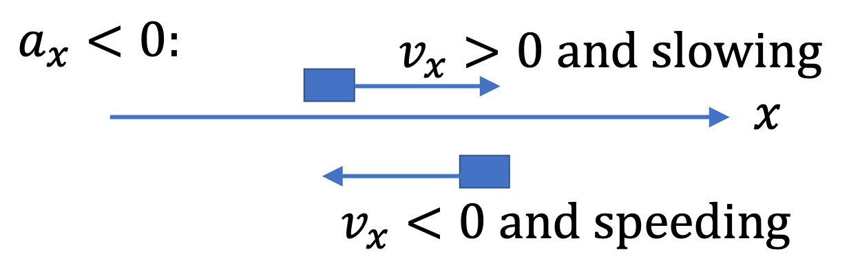
Sign conventions. We use a sign convention to follow the directions of velocity and acceleration. The justification of these sign conventions will become clear after you learn vectors. The following diagrams clarify the sign assignments of velocity and acceleration.

🔗

The velocity \(v_x \) is positive if object is moving in the direction of positive axis and negative if in the opposite direction.

🔗

Acceleration \(a_x \) is positive in two situations: if either \(v_x \) is positive and speeding up OR \(v_x \) is negative and slowing down.

🔗

Acceleration \(a_x \) is negative in two situations: if either \(v_x \) is negative and speeding up OR \(v_x \) is positive and slowing down.

🔗

Summary of Formulas

🔗

Constant Acceleration \(a_x\) during \(t_i\le t \le t_f\text{:}\)

🔗

\begin{align} \amp v_{f,x} - v_{i,x} = a_x \Delta t. \tag{2.21}\\ \amp \Delta x = v_{av,x} \Delta t.\tag{2.22}\\ \amp v_{av,x} = \dfrac{v_{i,x} + v_{f,x}}{2}.\tag{2.23}\\ \amp \Delta x = v_{i,x} \Delta t + \dfrac{1}{2}a_x\left(\Delta t \right)^2\tag{2.24}\\ \amp v_{f,x}^2 = v_{i,x}^2 + 2 a \Delta x\tag{2.25} \end{align}

🔗

Note that many of these symbols have subscript \(x\text{.}\) It is not necessary to use subscripts when it is understood that the motion is along one of the Cartesian axis. Therefore, we will often write them without verbose symbols: use \(a\text{,}\) \(v_0\text{,}\) \(v\text{,}\) \(x\text{,}\) \(t\) in place of \(a_x\text{,}\) \(v_{i,x}\text{,}\) \(v_{f,x}\text{,}\) \(\Delta x\text{,}\) \(\Delta t\text{,}\) respectively. Then, these equations look a lot simpler and remember them in this notation. Actually, you need to remember only the last two for solving problems, but remembering the first also often helps.

\begin{align} \amp v = v_0 + a t. \ \ \text{(** to memorize **)}\tag{2.26}\\ \amp x = v_{av} t.\tag{2.27}\\ \amp v_{av} = \dfrac{v_{0} + v}{2}.\tag{2.28}\\ \amp x = v_{0} t + \dfrac{1}{2}a t^2. \ \ \text{(** to memorize **)}\tag{2.29}\\ \amp v^2 = v_{0}^2 + 2 a x. \ \ \text{(** to memorize **)} \tag{2.30} \end{align}

🔗

Constant Speed \(v_s\) during \(t_i\le t \le t_f\text{:}\)

🔗

\begin{align} \amp |v_f| = |v_i| = v_{s} \tag{2.31}\\ \amp d = v_{s} \, \Delta t\tag{2.32} \end{align}

This says nothing about the acceleration since constant speed only says that absolute value of velocity is constant, but nothing about the direction of the velocity. Without the direction information about velocity, it is impossible to say anything about the acceleration, which depends on change in both magnitude and direction of velocity.

🔗

Example 2.60. Constant Acceleration of a Car from Zero Velocity.

A car can accelerate from zero velocity to \(30\text{ m/s} \) in \(2.5\text{ s}\text{.}\)

🔗

(a) What is the acceleration of the car?

🔗

(b) What is the average velocity of the car during the time of acceleration?

🔗

Answer.

(a) \(12.0\text{ m/s}^2\text{,}\) (b) \(15.0\text{ m/s}\text{,}\) (c) \(37.5\text{ m}\text{.}\)

🔗

Solution 1. a

From the change in velocity we find

\begin{equation*} a = \dfrac{v_f - v_i}{t} = \dfrac{30 \text{ m/s} - 0}{2.5\text{ s}} = 12 \text{ m/s}^2. \end{equation*}

🔗

Solution 2. b

Since acceleration is constant, average velocity will be average of initial and final velocities.

\begin{equation*} v_{av} = \dfrac{v_f + v_i}{2} = \dfrac{30 \text{ m/s} + 0}{2} = 15 \text{ m/s}. \end{equation*}

🔗

Solution 3. c

From average velocity and duration, we get the displacement to be

\begin{equation*} x_f - x_i = v_{av} t = 15 \text{ m/s} \times 2.5 \text{ s} = 37.5 \text{ m}. \end{equation*}

🔗

Example 2.61. Predicting the Final Velocity in a Constant Acceleration Motion.

A skier is coming down a steep slope with a constant acceleration \(a = 3.0\text{ m/s}^2\text{.}\) If the speed of the skier at the top of the hill was \(0 \text{,}\) what is his speed when he has skied a distance of \(40 \text{ m}\) down the hill? Ignore the bumps on the hill.

🔗

Answer.

\(15.5\text{ m/s}\text{.}\)

🔗

Solution.

Take the positive \(x \) axis to point down the hill. This will give us positive values for acceleration \(a_x\) and velocity \(v_x\text{.}\) For the sake of brevity, we will drop the coordinate subscript \(x \) from the symbols. From the problem statement, we can get the following.

\begin{equation*} a = 3.0\text{ m/s}^2,\ \ \Delta x = 40 \text{ m},\ \ v_i = 0,\ \ v_f = ? \end{equation*}

The “no-\(t\)-equation” is perfect for this and gives

\begin{equation*} v_f^2 = v_i^2 + 2 a \Delta x = 0 + 2 \times 3 \times 40 = 240. \end{equation*}

Taking square root of both sides gives two values

\begin{equation*} v_f = \pm 15.5\text{ m/s}. \end{equation*}

Its absolute value is speed \(v_{s}\text{.}\) Therefore

\begin{equation*} v_s = 15.5\text{ m/s}\text{.} \end{equation*}

🔗

Example 2.62. Stopping Distance in a Constantly Decelerating Situation.

Suppose maximum deceleration of a particular car is \(30.0\text{ m/s}^2\text{.}\) The car is moving at a steady pace at \(40.0\text{ m/s}\) on a straight road. The driver notices a deer on the road and applies the maximum brake right away. How far from the front of the car the deer must be if the car must stop before it hits the deer?

🔗

Answer.

\(26.7\text{ m}\text{.}\)

🔗

Solution.

Here, we are given that acceleration is in the opposite direction of initial velocity. So, if the initial velocity \(v_x \) is positive, the acceleration \(a_x\) will be negative. For brevity, I will drop \(x\) from the symbols. We have

\begin{equation*} v_i = 40.0 \text{ m/s}, \ \ v_f = 0, \ \ a = - 30.0 \text{ m/s}^2, \end{equation*}

and we are asked to find \(\Delta x\text{.}\) Using the “no-\(t\)-equation” we get (I will omit units in the calculations.)

\begin{equation*} v_f^2 - v_i^2 = 2 a \Delta x \rightarrow 0 - 40^2 = -2 \times 30 \times \Delta x. \end{equation*}

Note how the minus sign is necessary on the right for them to cancel out in this problem as it should. It should because, \(\Delta x\) should be positive since car is moving in the direction of positive \(x\) axis. Solving for \(\Delta x\) we get

\begin{equation*} \Delta x = 26.7\text{ m}. \end{equation*}

🔗

Example 2.63. Constant Acceleration Down an Incline.

Starting from rest a box slides down an incline at a constant acceleration of \(2\text{ m/s}^2\) pointed down the incline (not vertically down).

🔗

(a) Find speed of the box at \(t = 1.5\) sec.

🔗

(b) Find average velocity of the box between \(t = 0\) and \(t =1.5\) sec.

🔗

(d) Verify that the displacement during the \(1.5\)-sec interval is equal to the product of the average velocity for the interval and the time interval.

🔗

Answer.

(a) \(3.0\text{ m/s}\text{,}\) (b) \(1.5\text{ m/s}\text{,}\) (c) \(2.25\text{ m}\text{,}\) (d) \(2.25\text{ m}\text{.}\)

🔗

Solution 1. a

Let us point \(+x\) axis down the incline. This will give

\begin{equation*} a_x = + 2\text{ m/s}^2,\ \ v_{ix} = 0,\ \ \Delta t = 1.5\text{ sec}\equiv t. \end{equation*}

🔗

Therefore,

\begin{equation*} v_{fx} = v_{ix} + a_x t = 0 + 2\times 1.5 = 3.0\text{ m/s}. \end{equation*}

This gives final speed equal to \(3.0\text{ m/s}\text{.}\)

🔗

Solution 2. b

For constant acceleration, average velocity is just the average of initial and final velocities.

\begin{equation*} v_\text{av,x} = \dfrac{v_{ix} + v_{fx}}{2} = 1.5\text{ m/s}. \end{equation*}

🔗

Solution 3. c

The displacement from initial velocity and accl will be

\begin{equation*} \Delta x = v_{ix} t + \dfrac{1}{2}a t^2 = 0 + \dfrac{1}{2}\times 2\times 1.5^2 = 2.25\text{ m}. \end{equation*}

🔗

Solution 4. d

Using average velocity and duration we verify

\begin{equation*} \Delta x = v_\text{av,x}\, t= 1.5\times 1.5 = 2.25\text{ m}. \end{equation*}

🔗

Example 2.64. Deceleration of a Hockey Puck While Moving up an Incline.

A hockey puck is hit up an incline. The puck slows down at a constant acceleration of magnitude \(5\text{ m/s}^2\) and stops after \(1.2\) sec.

🔗

(a) Find the initial velocity, i.e. the velocity of the puck immediately after leaving the stick.

🔗

(b) How far up the incline does the puck go before coming to rest?

🔗

(d) Find the position of the puck at \(t = 0.5\text{ sec}\text{.}\)

🔗

Answer.

(a) \(6.0\text{ m/s}\) pointed up incline, (b) \(3.6\text{ m}\text{,}\) (c) \(3.5\text{ m/s}\) pointed up incline, (d) \(2.4\text{ m}\text{.}\)

🔗

Solution 1. a

Let \(+x\) axis be pointed up the incline. This makes \(a_x\) negative since puck’s velocity will be in the positive \(x\) direction and the puck will be slowing down. We will also drop \(x\) from the subscript of symbols and write \(t\) in place of \(\Delta t\text{.}\)

\begin{equation*} a = - 5.0\text{ m/s}^2,\ \ t = 1.2\text{ sec},\ \ v_{f} = 0. \end{equation*}

🔗

a From \(v_f = v_i + a t\) we get

\begin{equation*} v_{i} = v_{f} - a t = 0-(-5)\times 1.2 = 6.0\text{ m/s}. \end{equation*}

🔗

Solution 2. b

From \(\Delta x = v_{i} + \dfrac{1}{2}at^2\text{,}\) we get

\begin{equation*} \Delta x = 6\times 1.2 + \dfrac{1}{2}\times (-5)\times 1.2^2 = 3.6\text{ m}. \end{equation*}

🔗

Solution 3. c

Now, \(t=0.5\text{ s}\) and \(v_{f}\ne 0\text{.}\) We can use \(v_{i}\) found above to calculate \(v_{f}\text{.}\)

\begin{equation*} v_{f} = v_{i} + a t = 6.0 + (-5)\times 0.5 = 3.5\text{ m/s}. \end{equation*}

🔗

Solution 4. d

The displacement

\begin{align*} \Delta x \amp = \dfrac{v_{i} + v_{f}}{2}\, t\\ \amp = \dfrac{6 + 3.5}{2}\times 0.5 = 2.4\text{ m}. \end{align*}

You can also answer this part by

\begin{align*} \Delta x \amp = v_i t + \frac{1}{2} a t^2 \\ \amp = 6 \times 0.5 + 0.5\times (-5) \times 0.5^2 = 2.4\text{ m}. \end{align*}

🔗

Example 2.65. Constant Deceleration of a Skater.

A skater after an initial push glides with a constant deceleration. He comes to a stop after going \(120\) m in \(25\text{ sec}\text{.}\)

🔗

(a) Find his initial speed, i.e., immediately after the push.

🔗

(b) Find the deceleration during the free glide.

🔗

(d) How much distance did he cover in the last \(12.5\) sec?

🔗

Answer.

(a) \(9.6\text{ m/s}\text{,}\) (b) \(- 0.384\text{ m/s}^2 \text{,}\) (c) \(90\text{ m}\text{,}\) (d) \(30\text{ m}\text{.}\)

🔗

Solution 1. a

With \(+x\) axis in the direction of motion, we have

\begin{equation*} \Delta x = 120 \text{ m},\ \ v_{fx} = 0,\ \ \Delta t = 25\text{ s}\equiv t. \end{equation*}

Using \(\Delta x = v_{\text{av},x}\, \Delta t \) and \(v_{\text{av},x} = (v_{ix}+v_{fx})/2\text{,}\) we get

\begin{equation*} 120\text{ m} = \dfrac{v_{ix} + 0 }{2} \times 25\text{ s}. \end{equation*}

Therefore,

\begin{equation*} v_{ix} = 9.6\text{ m/s}. \end{equation*}

🔗

Solution 2. b

\begin{equation*} a_x = \dfrac{v_{fx} - v_{ix}}{\Delta t }= \dfrac{ 0 - 9.6 }{25} = - 0.384\text{ m/s}^2. \end{equation*}

🔗

Solution 3. c

Now, we have

\begin{equation*} v_{ix} = 9.6\text{ m/s},\ \ a_x = - 0.384\text{ m/s}^2,\ \ \Delta t = 12.5\text{ s}\equiv t. \end{equation*}

Therefore

\begin{align*} \Delta x \amp = v_{ix} t + \dfrac{1}{2}a_x t^2\\ \amp = 9.6 \times 12.5 + \dfrac{1}{2} \times (-0.384) \times 12.5^2 = 90\text{ m}. \end{align*}

🔗

Solution 4. d

\begin{equation*} \Delta x = 120\text{ m} - 90\text{ m} = 30\text{ m}. \end{equation*}

🔗

Example 2.66. Constant Acceleration on an Inclined Plane.

A truck is parked on an inclined slippery road. Suddenly, the brake fails and the truck starts to slide down the incline. You notice that starting from rest, the truck has picked up a speed of \(20.0 \) m/s over a period of \(30.0 \) seconds.

🔗

(a) Assuming constant acceleration, how far has the truck moved in this time?

🔗

(b) What is the acceleration of the truck?

🔗

Answer.

(a) \(300.0 \) m, (b) \(0.67 \text{ m/s}^2\) pointed down the incline.

🔗

Solution 1. a

Since we have a constant acceleration situation, it is easy to get average velocity from the initial and final velocities. Here, the initial velocity \(v_i = 0 \) since the truck was not moving initially, and the final velocity \(v_f = 20.0 \) m/s.

\begin{equation*} v_{av} = \dfrac{0 + 20.0}{2} = 10.0 \text{ m/s}. \end{equation*}

Therefore, the distance moved in \(t = 30.0 \) sec:

\begin{equation*} \Delta x = v_{av} t = 10.0 \text{ m/s} \times 30.0 \text{ s} = 300.0 \text{ m}. \end{equation*}

🔗

Solution 2. b

To get \(a \text{,}\) we just use the velocities and time given.

\begin{equation*} a = \dfrac{v_f - v_i }{t} = \dfrac{2}{3} \text{ m/s}^2. \end{equation*}

From the description, it is clear that truck’s speed is picking up. Hence, the direction of the acceleration is same as the direction in which the truck is moving, which is down the inclined road.

🔗

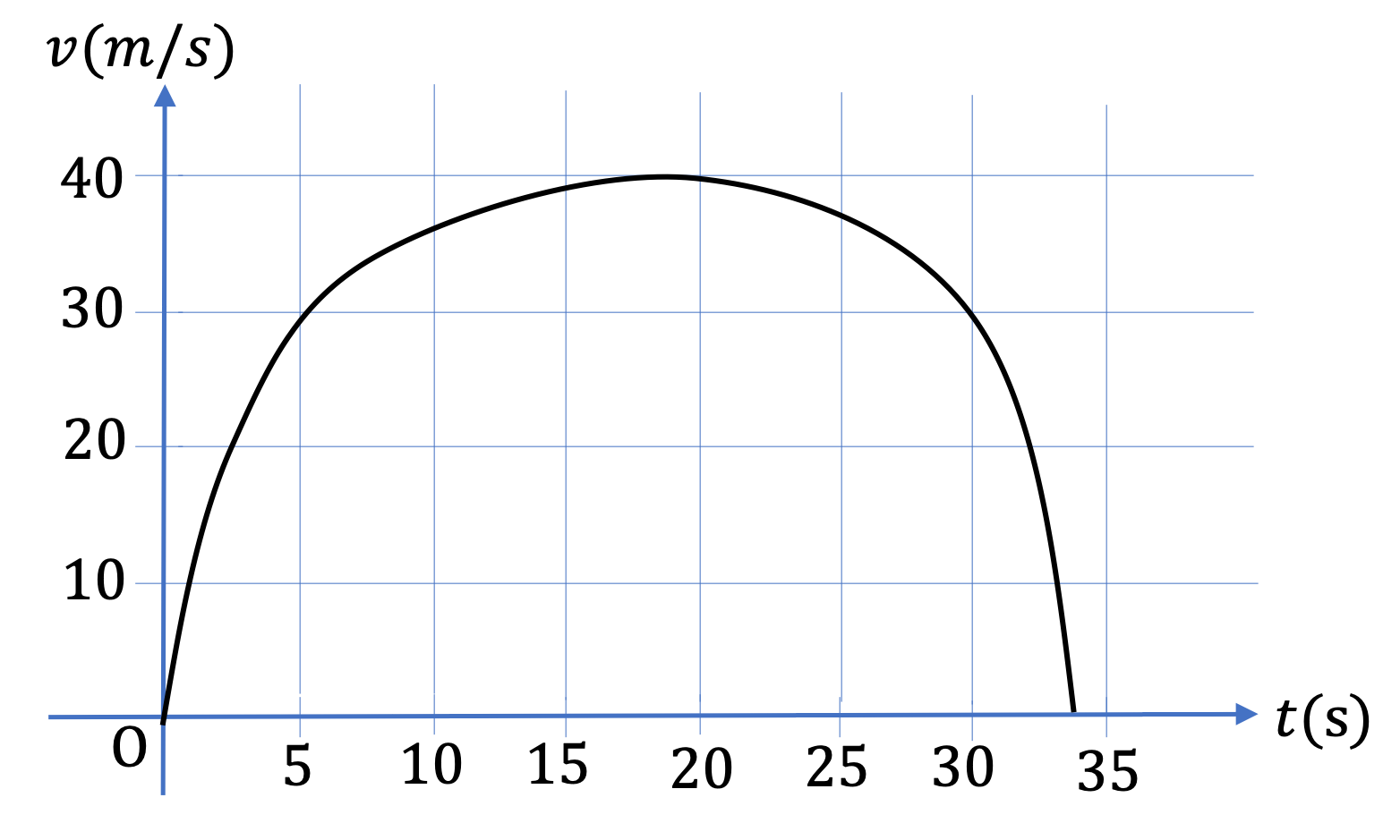
Example 2.67. Modeling a Varying Acceleration by Average Constant Acceleration.

A cheeta’s acceleration varies during its motion over a wide range. An example is given in Figure 2.68 below. Even though, the real-life situation is complicated, we can get a lot of physics by modeling the motion as if the motion was a constant acceleration motion, by replacing the varying acceleration by an average acceleration value. You would, of course not get the exact values, but your answer will be in the right ball park.

🔗

Suppose, the average acceleration of a cheetah between \(t=0 \) and \(t = 30\text{ sec}\) is \(2.2\text{ m/s}^2\text{.}\) If cheetah started out at rest, what will be (a) the distance traveled and (b) speed at \(t = 30\text{ sec}\text{?}\)

🔗

Answer.

(a) \(990\text{ m} \text{,}\) (b) \(66\text{ m/s} \text{.}\)

🔗

Solution 1. a

Since \(\Delta t\) and \(v_i \) are given to us, the following equation will give the displacement. Dropping \(x\) from subscript and writing \(t\) for \(\Delta t\text{.}\)

\begin{equation*} \Delta x = v_{i} t + \dfrac{1}{2} a_{\text{av}} t^2. \end{equation*}

With the numerical values given, we get

\begin{equation*} \Delta x = 0 + \dfrac{1}{2} \times 2.2\times 30^2 = 990\text{ m}. \end{equation*}

🔗

Solution 2. b

The velocity at the final instant can be obtained by

\begin{equation*} v_{f} = v_{i} + a_{\text{av}}\, t = 2.2\times 30 = 66\text{ m/s}. \end{equation*}

🔗

Exercises Exercises

1. Practice with a Friend: A Car Speeding Up a Ramp.

To merge into a highway traffic, a car accelerates on a ramp of length \(100\text{ m}\text{.}\) Starting from rest, the car makes it all the way to the end of the ramp in \(5.4\text{ sec}\text{.}\) Asuming the acceleration was constant, (a) what is the acceleration of the car? (b) what would be the speed of the car at the end of the ramp?

🔗

Answer.

\(6.86\,\text{m/s}^2\text{,}\)\(37\,\text{m/s}\text{.}\)

🔗

2. Practice with a Friend: A Skier Racing Down a Hill.

A skier is racing down a hill at a constant acceleration. Assume straightline motion. She covers a distance of \(100\,\text{m}\) in \(5\text{ s}\text{.}\) At the end she is going at speed \(30\text{ m/s}\text{.}\) (a) What was her acceleration? (b) What was her speed at the beginning?

🔗

Answer.

\(4\,\text{m/s}^2\text{,}\)\(10\,\text{m/s}\text{.}\)

🔗

Prev Top Next