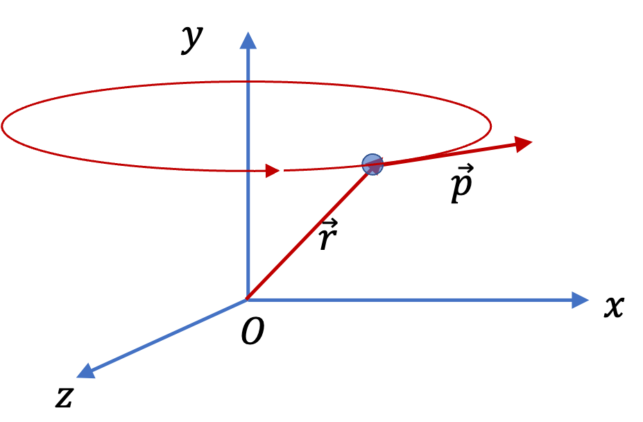
Consider a point particle of mass \(m\) at position \(\vec r\) from origin \(O\) is moving with speed \(\vec v\text{.}\) Then, angular momentum with respect to O is given by
\begin{equation}
\vec L = \vec r \times \vec p = m \vec r \times \vec v.\tag{10.7}
\end{equation}
We can write this also using angular velocity \(\vec \omega\text{.}\) Let us suppose that this coordinate system is the fixed coordinate system \(O'x'y'z'\) we have discussed in the last section. When discussing angular velocity we found that
\begin{equation*}
\vec v = \vec \omega \times \vec r.
\end{equation*}
Therefore, angular momentum can also be written as
\begin{equation}
\vec L = m \vec r \times (\vec \omega \times \vec r).\tag{10.8}
\end{equation}
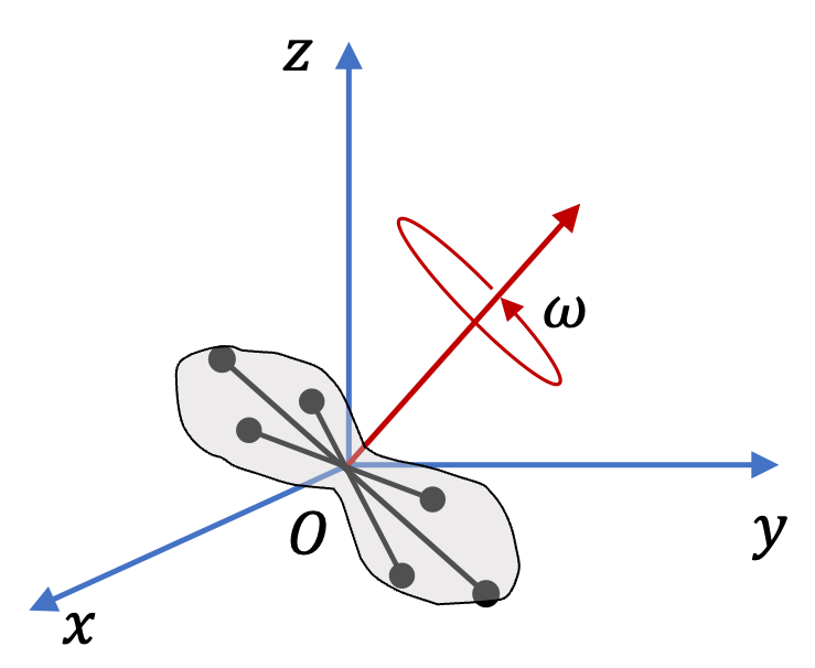
When a rigid body rotates, all of its particles rotate at the same angular velocity. But since different particles will be in different positions, their \(\vec r\) will be different. Say, we represent a rigid body by a collection of point particles of masses \(m_i\text{,}\) \(i = 1, 2, \cdots, N\text{.}\) Then, angular momentum of the body about O will be
\begin{equation}
\vec L = \sum_{i=1}^N m_i \vec r_i \times (\vec \omega \times \vec r_i).\tag{10.9}
\end{equation}
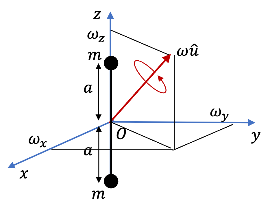
Expanding this in components can be done by writing \(\vec r\) and \(\vec \omega\) into components and carrying out the cross product.
\begin{equation*}
\vec r_i = x_i\,\hat i + y_i\,\hat j + z_i\,\hat k,\ \ \ \vec \omega = \omega_x\,\hat i + \omega_y\,\hat j + \omega_z\,\hat k.
\end{equation*}
Try to do this algebra to find the following expression for \(x\)-component \(L_x\text{.}\)
\begin{align*}
L_x \amp = \sum_i m_i \left( y_i^2 + z_i^2\right)\omega_x - \sum_i m_i x_i y_i \omega_y - \sum_i m_i x_i z_i \omega_z.
\end{align*}
The other components of angular momentum is easy to write down by analogy.
\begin{align*}
L_y\amp = \sum_i m_i \left( x_i^2 + z_i^2\right)\omega_y - \sum_i m_i y_i x_i \omega_x - \sum_i m_i y_i z_i \omega_z,\\
L_z\amp = \sum_i m_i \left( x_i^2 + y_i^2\right)\omega_z - \sum_i m_i z_i x_i \omega_x - \sum_i m_i z_i y_i \omega_y.
\end{align*}
Often it is helpful to drop the suffix that denumerates particles and just use the summation sign.
\begin{align}
\amp L_x = \sum m \left( y^2 + z^2\right)\omega_x - \sum m x y \omega_y - \sum m x z \omega_z.\tag{10.10}\\
\amp L_y = \sum m \left( x^2 + z^2\right)\omega_y - \sum m y x \omega_x - \sum m y z \omega_z.\tag{10.11}\\
\amp L_z = \sum m \left( x^2 + y^2\right)\omega_z - \sum m z x \omega_x - \sum m z y \omega_y.\tag{10.12}
\end{align}
Often, we write relation between components of \(\vec L\) and \(\vec \omega\) using a matrix multiplication notation.
\begin{equation}
\begin{pmatrix}
L_x\\
L_y\\
L_z
\end{pmatrix} =
\begin{pmatrix}
\sum m \left( y^2 + z^2\right) \amp - \sum m x y \amp - \sum m x z\\
- \sum m y x \amp \sum m \left( x^2 + z^2\right) \amp - \sum m y z\\
- \sum m z x \amp - \sum m z y \amp \sum m \left( x^2 + y^2\right)
\end{pmatrix}
\begin{pmatrix}
\omega_x\\
\omega_y\\
\omega_z
\end{pmatrix} \tag{10.13}
\end{equation}
We write this equation in a formal way by denoting the quantities in the matrix by bold letter \({\bf I}\text{.}\)
\begin{equation}
\vec L = {\bf I}\, \vec \omega.\tag{10.14}
\end{equation}
Unlike vectors \(\vec L\) and \(\vec \omega\text{,}\) which have three Cartesian components, \({\bf I}\) has nine components. We call \({\bf I}\) moment inertial tensor. There are other tensor type properties in physics such as electic conductivity and refractive index tensors. The components of tensor are denoted by two subscripts corresponding to the axes. Thus,
\begin{align}
\amp I_{xx} = \sum m \left( y^2 + z^2\right),\ \ I_{xy} = - \sum m x y,\ \ I_{xz} = - \sum m x z\tag{10.15}\\
\amp I_{yx} = - \sum m y x,\ \ I_{yy} = \sum m \left( x^2 + z^2\right) ,\ \ I_{yz} = - \sum m y z\tag{10.16}\\
\amp I_{zx} = - \sum m z x,\ \ I_{zy} = - \sum m z y,\ \ I_{zz} = \sum m \left( x^2 + y^2\right) \tag{10.17}
\end{align}
The diagonal components, \(I_{xx}\text{,}\) \(I_{yy}\text{,}\) \(I_{zz}\) are called moments of inertia about \(x\text{,}\) \(y\text{,}\) and \(z\) axes respectively. The off-diaginal components do not have such simple interpretations.
If a body is regarded as continuous, the sum in these definitions become integrals. To go from sum over masses to integrals over space, we replace \(m\) by \(\rho dV\text{,}\) where \(\rho\) is the density, \(dV\) is a volume element. In the case of two-dimensional structure, you will have area element \(dA\) and in the case of a one-dimensional structure it will be just a size \(ds\text{.}\) Thus, the diagonal elment \(I_{zz}\) will be
\begin{equation}
I_{zz} = \int\, \rho \, \left( x^2 + y^2\right)\, dV,\tag{10.18}
\end{equation}
and off-diagonal element \(I_{zx}\) will be
\begin{equation}
I_{zx} = -\int\, \rho \, z x \, dV.\tag{10.19}
\end{equation}
The other components of \({\bf I}\) will be obtained in a similar way.
From the matrix representation of \({\bf I}\text{,}\) it is obvious that it is a symmetric matrix. We say that moment of inertia is a symmetric tensor. Since symmetric matrices can always be diagonalized, there is a choice of direction of the body-attached axes so that off-diagonal elements turn out to be zero. We call these axes principal axes. In principal axes we will have only three non-zero moment of inertia components; in that case, we just denote them by simpler symbols, \(I_1\text{,}\) \(I_2\text{,}\) \(I_3\text{.}\)
\begin{equation*}
{\bf I} =
\begin{pmatrix}
I_1 \amp 0 \amp 0\\
0 \amp I_2 \amp 0\\
0 \amp 0 \amp I_3
\end{pmatrix}
\end{equation*}